These are example input scripts for regularrized LLG simulations, the full API can be found here.

Key points

1. The regularization works for Bloch points. In the case of smooth magnetic vector fields, the use of the S3-model is pointless.

2. The Kappa parameter has units of magnetocrystalline anisotropy and has to be defined (see examples below).

3. To run simulations with the rLLG equation, one has to call SetSolver(8), which corresponds tothe RK45 method with adaptive time step

Bloch point motion in an Fe nanowire

// Discretization
sc := 1;
nx := 16*sc;    nz := 256*sc;       
Lx := 35.0e-9;  Lz := 1200.0e-9
dx:= Lx/nx;     dz:= Lz/nz;
SetMesh(nx, nx, nz, dx, dx, dz, 0, 0, 0)
MinimizerStop = 1e-5;

// Wire geometry
setgeom( circle(1.0*Lx) )

// Material parameters for Fe
EnableDemag = true
Ms := 1700e3;   Msat = Ms;  //Magnetization saturation
A := 21.0e-12;  Aex = A     //Exchange stiffnes
B_ext = vector(0,0,0)       //External field
Kappa = 0.5e6;              //kappa-paramter in the S3-model [anisotropy units]

// Initial state: two domains (Up and Down)
// separated by a domain wall containing a Bloch point
m = uniform(0, 0, 1)

defregion(1, zrange(-0.5*Lz, -0.05*Lz))
defregion(2, zrange(0.05*Lz, 0.5*Lz))
defregion(3, zrange(-0.05*Lz, 0.05*Lz))

m.setRegion(1, uniform(0.1, 0, 1))
m.setRegion(3, vortex(-1, -1) )
m.setRegion(2, uniform(0.1, 0, -1))

// Relaxation with standard Mumax methods
relax(); minimize(); save(m)

// Relaxation within the S3-model
alpha = 1.0;//Damping
SetSolver(8)
run(1e-9)
save(m)

// Dynamics with the regularized LLG
alpha = 0.01;//Damping
B_ext = vector(0,0,1e-3)
tableautosave(10e-13)
autosave(m, 0.1e-9)
run(100e-9)
    

output

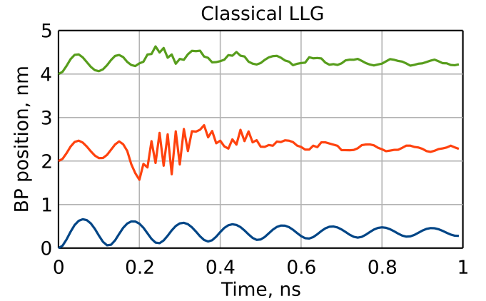
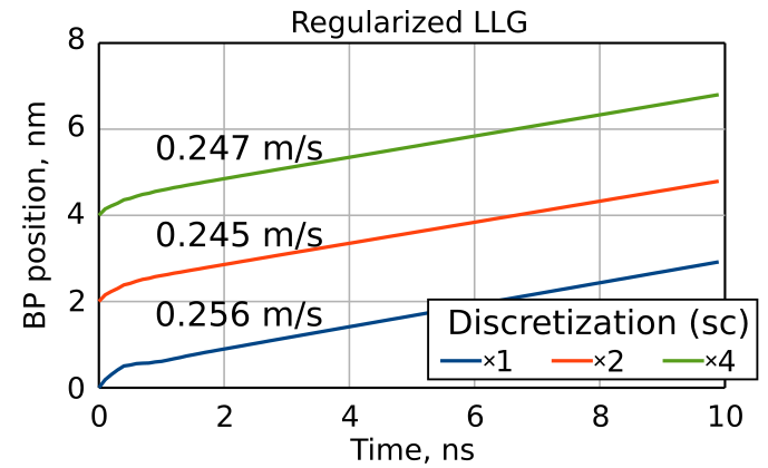
Performing simulations for different cuboid sizes (sc = 1, 2, 4) and extracting the Bloch point's position, we summarize the obtained results for classical and regularized LLG equations below:

Current-induced motion of a chiral bobber

OutputFormat = OVF2_BINARY
Ms := 384e3;  Msat = Ms             //Magnetization saturation
A := 4.0e-12; Aex = A               //Exchange stiffnes
LD := 70.0e-9;                      //Spin-spiral period for FeGe
D := 4.0 * pi * A / LD              //DMI strength
Dbulk = D
BD := D * D / (2 * A * Ms)
MinimizerStop = 1e-5
Xi = 0.25
alpha = 1.0
L := 2.0 * LD
n := 64
SetGridSize(n, n, n)
dl := L / n
SetCellSize(dl, dl, dl)
SetPBC(1, 1, 0)

EnableDemag = false
B := 0.7 * BD                       //External magnetic field
B_ext = vector(0, 0, B)

Kappa = (1.0e-4) * D * D / (2 * A)  //kappa-paramter in the S3-model [anisotropy units]

// Initial state: chiral bobber within cone phase background
m = Conical(vector(0,0,2*PI/LD), vector(0,0,1), PI/4)
m.setInShape(cylinder(LD, L).transl(0, 0,0.5*L),BlochSkyrmion(1, -1).transl(0, 0,0.5*L))

// Relaxation with standard Mumax methods
relax(); minimize(); save(m);
 
// Relaxation within the S3-model 
//(comment this code to simulate standard LLG)
alpha = 1.0;//Damping
SetSolver(8)
run(1e-9)
save(m)

//Dynamics with Zhang-Li torque
alpha = 0.05
tableautosave(10e-12)
autosave(m, 1e-9)
J = vector(-(1-(1+exp(2e9*(-1e-9)))/(1+exp(2e9*(t-1e-9))))*3e10, 0, 0) 
run(100e-9)

    

output

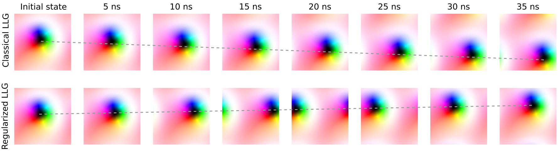
Performing simulations with the standard and regularized LLG equations, we can compare chiral bobber motion. The dashed gray line shows the trajectory of the bobber from which we can estimate the skyrmion Hall angle. This angle is negative in the former case (in disagreement with the Thiele equation) and positive in the latter case (in agreement with the Thiele equation).