Note that this is an extension and is not available in the original mumax3 code!
These are example input scripts for gneb simulations, the full API can be found here.
1. The entire system is simulated at once, and all images are placed one on top of another along the z-axis.
Meaning, if a system is discretized into Nx*Ny*Nz cuboids and we want to simulate Noi images, the total system size is Nx*Ny*(Nz*Noi).
2. Geom() is not implemented for the GNEB simulations.
One must use the DefRegionCell() function to simulate various shapes. Region number 255 is non-magnetic.
3. Custom fields are not compatible with the GNEB simulations.
4. For simulations with demagnetizing fields enabled, the corresponding kernel has to be precomputed with an additional mumax3 script (see examples below).
The stored kernel in ~/tmp/ directory will be used for GNEB simulations. Note that the number of cuboids, images, and cuboid size must be the same.
5. The GNEB method is very sensitive to the initial guess for the path between given two states.
Approaches to generate such a guess represent a separate topic and won't be covered here.
Partially, this was discussed in Section 4: 2D skyrmion homotopies.
The initial state can be defined in various ways:
1) with a standard mumax3 function SetCell();
2) using a stored texture m.LoadFile("FileName.ovf");
3) using linear intepolation between two given states, m.InterpolatePath(”State1.ovf”, ”State2.ovf”, Noi).
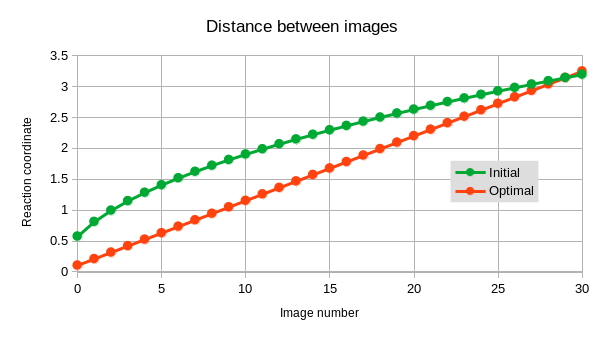
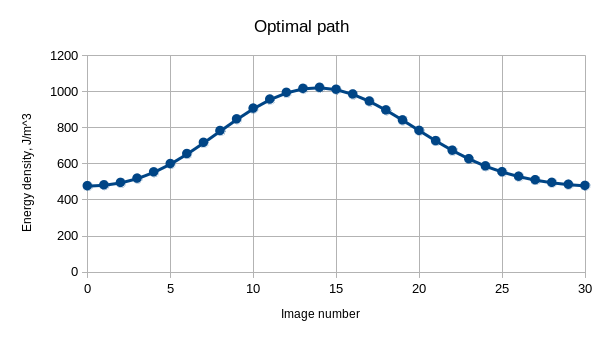
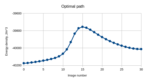
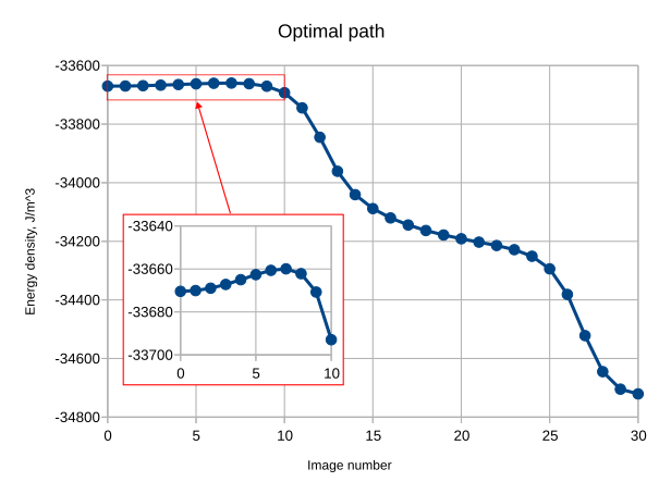
The output file table.txt contains four columns: image number, image energy, image torque, and reaction coordinate (Euclidean distance).
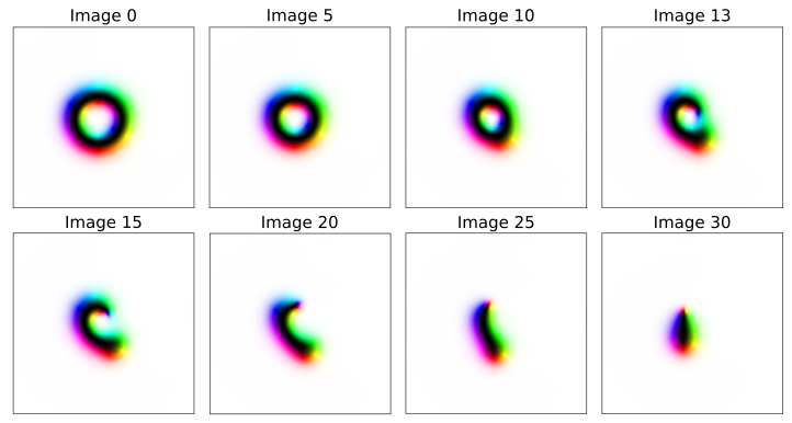
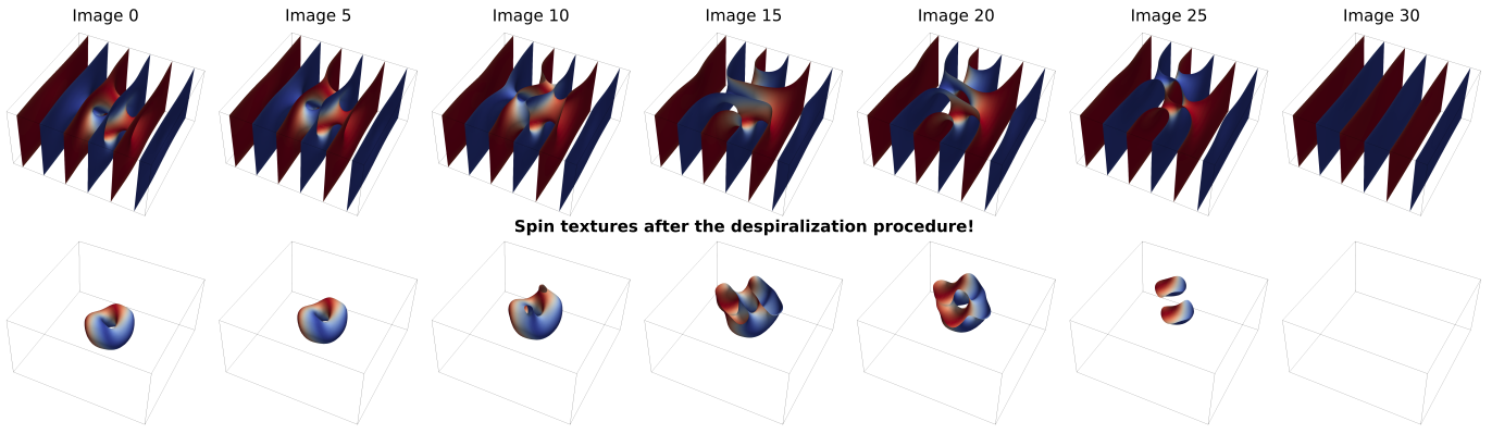
The magnetization texture of each image can be obtained by calling save(m) or SavePath(m, Noi).
nx := 1; ny := 1; nz := 1; noi := 31; //Discretization
dx := 1e-9; // cuboid size
SetMeshGNEB(nx, ny, nz*noi, noi , dx, dx, dx, 0, 0, 0, 1 , 0 )
// Material parameters
EnableDemag = false
Ms := 200e3;
Msat = Ms
Ku1 = 1.0 //anisotropy
anisU = vector(0, 0, 1)
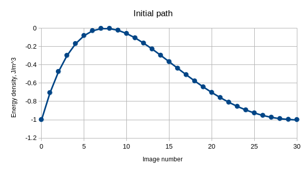
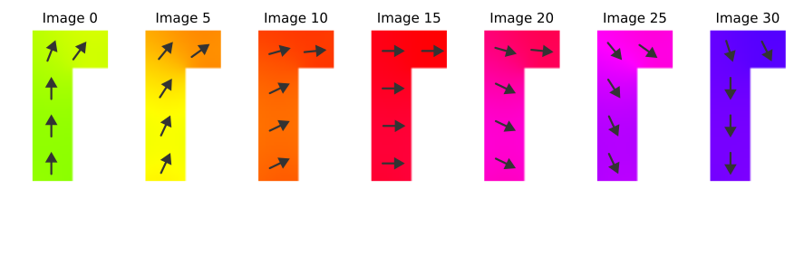
//Initial state
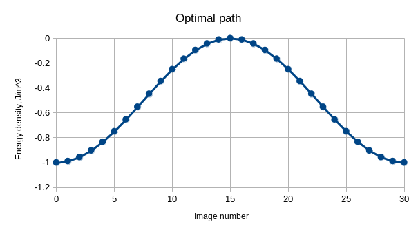
// we start with a non-uniform rotation
// solution will be a uniform rotation
for i:=0; i<noi; i++{
Th := pi*sqrt(i/(noi-1));
mnew := vector(0, sin(Th), cos(Th));
m.SetCell(0, 0, i, mnew);
}
save(m) //save initial state
//GNEB relaxation parameters
k_force = 1.0e2 // spring force constant
MaxIter = 1e7 // Maximal number of iterations
WritingIter = 100 // how often write to table.txt
MaxForce = 5e-6 // tolerance for forces
StepSize = 3e-3 // step size in VPO method
VPOminimize() // run VPO
save(m) // save final state
nx := 32; ny := 64; nz := 1; noi := 31; //Discretization
dx := 4e-9;         // cuboid size
SetMeshGNEB(nx, ny, nz, noi , dx, dx, dx, 0, 0, 0, 0, 0 )
// Material parameters
EnableDemag = true
Msat = 200e3;
MaxIter = 1         // Maximal number of iterations
VPOminimize()       // run VPO
//Did not use cached kernel: open /tmp/mumax3kernel_[32 64 1]_[0 0 0]_[4e-09 4e-09 4e-09]_6_0 0.ovf: no such file or directory
// Calculating demag kernel 0 %
// Calculating demag kernel 100 %
//Cached kernel: /tmp/mumax3kernel_[32 64 31]_[0 0 0]_[4e-09 4e-09 4e-09]_6_
nx := 32; ny := 64; nz := 31; noi := 31; //Discretization
dx := 4e-9;         // cuboid size
SetMeshGNEB(nx, ny, nz, noi , dx, dx, dx, 0, 0, 0, 1 , 0 )

// Material parameters
EnableDemag = true
Msat = 200e3;
Aex = 13e-12;

// Define shape and generating initial state
for k:=0; k<noi; k++{
    for i:=0; i<nx; i++{
        for j:=0; j<ny; j++{
            if(i>nx/2 && j < 3*ny/4){
                DefRegionCell(255, i, j, k)
            }else{
                DefRegionCell(0, i, j, k);
                //uniform rotation:
                Th := pi*(k+5)/(noi+7);
                mnew := vector(sin(Th), cos(Th), 0);
                m.SetCell(i, j, k, mnew);
            }
        }
    }
}
Aex.setregion(255, 0)
NoDemagSpins.SetRegion(255, 1)
m.setRegion(255, uniform(0,0,1))

// GNEB relaxation parameters
k_force =  1.0e2    // spring force constant
MaxIter = 1e7       // Maximal number of iterations
WritingIter = 100   // how often write to txt file0
MaxForce = 5e-7     // tolerance for forces
stepsize = 3e-2     // step size in VPO method
VPOminimize()       // run VPO
save(m)             // save final state
// system discretization
setgridsize(32, 64, 31)
setcellsize(4e-9,4e-9,4e-9)

//loading relaxed path
m.LoadFile("G-shape.ovf")
//saving each image as a separate ovf file
SavePath(m, 31)
nx := 256; ny := 256; nz := 31; noi := 31; //Discretization
dx := 1.09375e-9; // cuboid size to have 4LD by 4LD system
SetMeshGNEB(nx, ny, nz, noi , dx, dx, dx, 1, 1, 0, 1, 0)

// Material parameters
EnableDemag = false
Ms := 384e3;    Msat = Ms;
A  := 4.0e-12;  Aex = A;
LD := 70e-9;        //spin-spiral period in FeGe
D  := 4.0*pi*A/LD; Dbulk = D
BD := D*D/(2*A*Ms); //saturation field
B_ext = vector(0, 0, 0.7*BD)

//Initial state
m = uniform(0, 0, 1)
m = BlochSkyrmion(1,-1).scale(7,7,1)
m.setInShape(cylinder(1*LD, Noi*dx), BlochSkyrmion(-1,1).scale(2,2,1))

//adding a local magnetic field
//to initiate domain wall breaking
mask := newVectorMask(Nx, Ny, Nz)
for k:=0; k<Nz; k++{
    for i:=25; i<Nx/2; i++{
        for j:=0; j<Ny/2; j++{
            mask.setVector(Nx/2 + i, Ny/2 + j, k, vector(0, 0, 19*sqrt(1.0*k+1)))
        }
    }
}
B_ext.add(mask, BD)

//Relaxation parameters
DoRelax = 1;        // relax all images separately
MaxIter = 3e3       // Maximal number of iterations
MaxForce = 5e-7     // tolerance for forces
stepsize = 3e-2     // step size in VPO method
VPOminimize()       // run VPO
save(m)             // save final state
nx := 512; ny := 512; nz := 31; noi := 31; //Discretization
dx := 0.5*1.09375e-9; // cuboid size
SetMeshGNEB(nx, ny, nz, noi , dx, dx, dx, 1, 1, 0, 1, 0)

// Material parameters
EnableDemag = false
Ms := 384e3;    Msat = Ms;
A  := 4.0e-12;  Aex = A;
LD := 70e-9;        //spin-spiral period in FeGe
D  := 4.0 * pi * A / LD; Dbulk = D
BD := D*D/(2*A*Ms); //saturation field
B_ext = vector(0, 0, 0.63*BD)

//Initial state
m.LoadFile("ini_path.ovf")

//GNEB relaxation parameters
k_force =  1.0e1        // spring force constant
MaxIter = 1e7           // Maximal number of iterations
WritingIter = 100       // how often write to txt file0
MaxForce = 5e-8         // tolerance for forces
stepsize = 3e-2         // step size in VPO method
VPOminimize()           // run VPO
save(m)                 // save final state
nx := 64; ny := 64; nz := 32; noi := 31; // Discretization
dx := 210e-9/64;            // cuboid size corresponds to box 3LDx3LDx2LD
SetMeshGNEB(nx, ny, nz*noi, noi , dx, dx, dx, 1, 1, 0, 0, 1)

// Material parameters for FeGe
EnableDemag = false
Ms := 384e3;    Msat = Ms;   // Magnetization saturation
A  := 4.0e-12;  Aex = A;     // Exchange constant
LD := 70e-9;                 // spin-spiral period
D  := 4.0*pi*A/LD; Dbulk = D // DMI constant

//Initial state

// Running this part of code is a bit slow.
// It makes sense to save this spin texture,
// and then just use the stored state.

for q:=0; q<noi; q++{
    img := 0.8*q/(noi-1)
    for k:=0; k<nz; k++{
        for i:=0; i<nx; i++{
            for j:=0; j<ny; j++{
                x   := -1.5 + 3.0*i/(nx-1) + 1e-8;
                y   := -1.5 + 3.0*j/(ny-1) + 1e-8;
                z   := -1.0 + 2.0*k/(nz-1) + 1e-8 - img;
                r   := sqrt(x*x + y*y + z*z);
                // ansatz from: doi.org/10.3389/fphy.2023.1201018
                G   := 2.0*atan(exp(-2.0*r)/r);
                mx  := y*sin(2.0*G)/r + 2.0*sin(G)*sin(G)*x*z/(r*r);
                my  := x*sin(2.0*G)/r - 2.0*sin(G)*sin(G)*y*z/(r*r);
                mz  :=   cos(2.0*G)   + 2.0*sin(G)*sin(G)*z*z/(r*r);
                // spiralization
                phi  := 2*pi*y
                mnew := vector( mx*cos(phi)+mz*sin(phi), my,
                                mz*cos(phi)-mx*sin(phi));
                m.SetCell(i, j, k + nz*q, mnew);
            }
        }
    }
}
save(m)
//m.LoadFile("ini_state.ovf")

//GNEB relaxation parameters
k_force =  1.0e3    // spring force constant
MaxIter = 1e7       // Maximal number of iterations
WritingIter = 100   // how often write to txt file
MaxForce = 1e-8     // tolerance for forces
stepsize = 2e-2     // step size in VPO method
VPOminimize()       // run VPO

save(m)             // save final state
SavePath(m, noi)    // save as separate files
nx := 64; ny := 64; nz := 32; noi := 31; //Discretization
dx := 210e-9/64;
SetMesh(nx, ny, nz, dx, dx, dx, 1, 1, 0)

//Despiralization:
// transforms spiral state (cos(q*y), 0, sin(q*y))
// into the saturated state (0,0,1)
for i:=0; i<noi; i++{
    s := Sprintf("image%d.ovf", i)
    m.LoadFile(s)
    for j:=0; j<ny; j++{
        y    := -1.5 + 3.0*j/(ny-1) + 1e-8;
        phi  := -2*pi*y
        for k:=0; k<nz; k++{
            for i:=0; i<nx; i++{
            m0   := m.GetCell(i,j,k);
            mnew := vector(m0[0]*cos(phi) + m0[2]*sin(phi), m0[1],
                           m0[2]*cos(phi) - m0[0]*sin(phi))
            m.SetCell(i, j, k, mnew);
        }
    }
}
save(m)
}